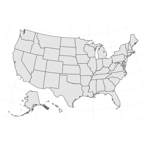
class: center, middle, inverse, title-slide # Geospatial Visualization using R ## Part 5: Ways to Output Maps ### Bhaskar V. Karambelkar ### 2017/07/04 --- # Options to Display Maps - Display in your R session's graphics device. - Save to a static image in one of the raster formats.<br/><br/>`.jpg` uses lossy & `bmp`/`.tiff`/`.png` use lossless compression. (TIFF are huge!) - Save to a static image in a vector format.<br/><br/>SVG is the most popular and supported by major browsers. - Save a set of incremental images in a `gif` or `mp4` file for animation. - Display statically in a document (PDF/Word/HTML). - Display interactively (see `leaflet`) and/or dynamically (see `shiny`) in web pages/applications. --- # Save Static Images - If using base R plotting, open a device for you format, plot and close device. ```r * png(filename="plot-01.png", width=800, height=600, units='px') plot(maps::map()) dev.off() ``` - If using ggplot2 based plotting, use `ggsave`. ```r library(ggplot2); g <- ggplot() + geom_sf(data=albersusa::usa_sf()) + ggthemes::theme_map() + coord_sf(crs = albersusa::us_aeqd_proj) * ggsave('plot-02.png', g, device = 'png') ``` - You can customize the device using `png()`|`pdf()`|`jpg()`|`svg()`|`tiff()` functions. - `Cairo` package provides graphics devices for high-quality production-ready images. --- # Raster v/s Vector .pull-left[ .center[ ### Raster Image ] <!-- --> ] .pull-right[ .center[ ### Vector Image ] <!-- --> ] --- # Animations - `gganimate::gganimate_save()` - `animation::save*()` - Both these packages support multiple output formats such as `GIF` / `mp4` etc., but depend on external programs/libraries like `ffmpeg`, `imagemagick` etc. <img src='animation-01.gif' width='400px' style="display: block;margin-left: auto;margin-right: auto" /> --- # Display statically in PDFs/HTMLs/Word Docs - `knitr` and `rmarkdown` packages is all you need. Plus `pandoc` command-line utility. <pre><code class="r hlsjs remark-code"> ```{r ggplot-01, fig.width=8, fig.height=6, fig.align='center'} library(ggplot2) ggplot() + geom_sf(data=albersusa::usa_sf()) + ggthemes::theme_map() + coord_sf(crs = albersusa::us_aeqd_proj) ``` </code></pre> - When it doubt, consult `knitr` [chunk options](https://yihui.name/knitr/options) and [hooks](https://yihui.name/knitr/hooks/), and [rmarkdown](http://rmarkdown.rstudio.com/lesson-1.html) manuals. - Confused still ? Zev Ross has an excellent [blog post](http://zevross.com/blog/2017/06/19/tips-and-tricks-for-working-with-images-and-figures-in-r-markdown-documents/) explaining the details. - Lastly, for speedier rendering cache chunk outputs. Somewhere at the start <pre><code class="r hlsjs remark-code"> ```{r setup, include=FALSE} knitr::opts_chunk$set(cache = TRUE) ``` </code></pre> --- # Dynamic Maps - Using `shiny` in applications, or rmarkdown HTML documents with shiny backend. - These maps are dynamic, as in they can change as per user input, but not really interactive, as in a user cannot interactively explore them. - This is not my code! I found it on the [intertubes](https://gallery.shinyapps.io/shiny-salesman/). <iframe src="https://gallery.shinyapps.io/shiny-salesman/" height="350px" width="900px" /> --- # Interactive Maps - These make sense in a web environment. Here a user can interact with the map. e.g. zoom in/out, pan, toggle stuff, get more information with popups and labels etc. - `plotly` is probably the easiest way for interactive maps. Can wrap most `ggplot2` maps in to interactive versions. - `leaflet` + related packages for extreme control and flexibility. - `rbokeh` / `highcharter` too have mapping capabilities. - All the above are instances of `htmlwidgets`. R wrapper packages for JavaScript based visualization APIs. - `widgetframe` package allows you to wrap a widget in an iframe for better display in HTML outputs. - `htmlwidgets` can talk to each other using `crosstalk` (w/o needing `shiny`). - For wizzard level mapping you can combine `htmlwidgets` + `crosstalk` + `shiny`. --- class: inverse middle # Part 5: The End! Continue to [Part 6: Static Maps](06-Static_Maps.html) .footnote[Restart [Part 5: Ways to Output Maps](05-Ways_to_Output_Maps.html)]